Conditional Formatting

Looking at a huge amount of data and wondering where the highlights are? Who has the highest (or lowest) score, what the top five are, etc.? Do you want to create your own data heat map?

Excel's Conditional Formatting will do everything from put a border around the highlights to color coding the entire table. It will even build a graph into each cell so you can visualize the top and bottom of the range of numbers at a glance.

Use the Highlighted Cells Rules sub-menu to create more rules to look for things, such as text that contains a certain string of words, recurring dates, duplicate values, etc. There's even a greater than/less than option so you can compare number changes.

You can apply conditional formatting to a range of cells (either a selection or a named range), an Excel table, and in Excel for Windows, even a PivotTable report.

Expert Tip - Use the Format Painter to copy conditional formatting to other cells

 

Types of Conditional Formatting Options

There are 5 types of conditional formatting visualizations available:

• Background Color Shading (of cells)
• Foreground Color Shading (of fonts)
• Data Bars
• Icons (which have 4 different image types)
• Values

Apply conditional formatting

1. Select the range of cells, the table, or the whole sheet that you want to apply conditional formatting to.

2. On the Home tab, click Conditional Formatting.

   

3. Do one of the following:

   To highlight	Do this
   Values in specific cells. Examples are dates after this week, or numbers between 50 and 100, or the bottom 10% of scores.	Point to Highlight Cells Rules or Top/Bottom Rules, and then click the appropriate option.
   The relationship of values in a cell range. Extends a band of color across the cell. Examples are comparisons of prices or populations in the largest cities.	Point to Data Bars, and then click the fill that you want.
   The relationship of values in a cell range. Applies a color scale where the intensity of the cell's color reflects the value's placement toward the top or bottom of the range. An example is sales distributions across regions.	Point to Color Scales, and then click the scale that you want.
   A cell range that contains three to five groups of values, where each group has its own threshold. For example, you might assign a set of three icons to highlight cells that reflect sales below $80,000, below $60,000, and below $40,000. Or you might assign a 5-point rating system for automobiles and apply a set of five icons.	Point to Icon Sets, and then click a set.

 

 

 

To Clear/Remove Conditional Formatting - ​​​Clear Worksheet    

• On the Home tab, click Conditional Formatting > Clear Rules > Clear Rules from Entire Sheet.

 

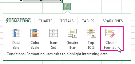
To Clear/Remove Conditional Formatting - Clear a Range of Cells

1. Select the cells that contain the conditional formatting.

2. Click the Quick Analysis Lens  button that appears to the bottom right of the selected data.

   Notes:  Quick Analysis Lens will not be visible if:

   • All of the cells in the selected range are empty, or

   • There is an entry only in the upper-left cell of the selected range, with all of the other cells in the range being empty.

3. Click Clear Format.

   

 

Find and remove the same conditional formats throughout a worksheet

1. Click on a cell that has the conditional format that you want to remove throughout the worksheet.

2. On the Home tab, click the arrow next to Find & Select, and then click Go To Special.

3. Click Conditional formats.

4. Click Same under Data validation. to select all of the cells that contain the same conditional formatting rules.

5. On the Home tab, click Conditional Formatting > Clear Rules > Clear Rules from Selected Cells.