Suppose you have a spreadsheet that is arranged into two rows. This arrangement would quickly become unwieldy if more columns were added. It would be better to rearrange this data into two columns instead:

Luckily, you don't have to rearrange each cell by hand. Excel can do it automatically using a feature called Transpose, which is available when copying and pasting data.
Step 1: Select blank cells
First select some blank cells. But make sure to select the same number of cells as the original set of cells, but in the other direction. For example, there are 8 cells here that are arranged vertically:

So, we need to select eight horizontal cells, like this:

This is where the new, transposed cells will end up.
Step 2: Type =TRANSPOSE(
With those blank cells still selected, type: =TRANSPOSE(
Excel will look similar to this:
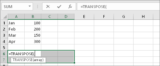
Notice that the eight cells are still selected even though we have started typing a formula.
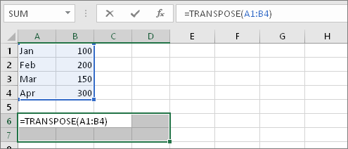
Step 3: Type the range of the original cells.
Now type the range of the cells you want to transpose. In this example, we want to transpose cells from A1 to B4. So the formula for this example would be: =TRANSPOSE(A1:B4) -- but don't press ENTER yet! Just stop typing, and go to the next step.
Excel will look similar to this:
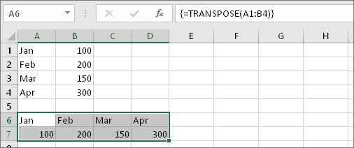
Step 4: Finally, press CTRL+SHIFT+ENTER
Now press CTRL+SHIFT+ENTER. Why? Because the TRANSPOSE function is only used in array formulas, and that's how you finish an array formula. An array formula, in short, is a formula that gets applied to more than one cell. Because you selected more than one cell in step 1, the formula will get applied to more than one cell. Here's the result after pressing CTRL+SHIFT+ENTER: